This article describes the AES reference implementation that I wrote in Haskell. I have implemented this algorithm half a dozen times over my career, for use in FIPS compliant implementations, for use in embedded systems, and even for use as a building block for more interesting things. This implementation is destined to be used for such an interesting project, which we will talk about during the next blog entry. First, we need an AES algorithm. AES is an interesting algorithm that combines some of the common elements typical of encryption, such as Confusion and Diffusion and Abstract Algebra, in this case Galois Field Theory. AES is based on the Rijndael block cipher, but with specific tunings as decided by NIST. Rijndael is a more general algorithm. This article stays close to AES, but implements tunable parameters which takes the algorithm away from the standard by adding back some ideas found in the original cipher. Since the point of this implementation is to build a parameterized PRNG and not to build an encryption system, I think this is a decent trade-off.
First, I should crush some expectations. This implementation of the cipher is a reference implementation. It should not be used in a production environment, or for any purpose where security is important. This only implements ECB mode, which is the weakest encryption mode. ECB is a building block for more interesting things, but it cannot be used on its own without opening one up to many terrible attacks. Also, this implementation is not timing resistant. Although it uses table lookups for the important operations, Haskell is not a low-level enough language to make any claims about cache coherency or even how operations are performed by the CPU. This implementation will leak key details through timing attacks. Finally, this implementation is garbage collected. Secret data will exist throughout RAM for an indeterminate amount of time. On most platforms, a Haskell process runs in user space, and its RAM could be accessible by other processes running on the system. Key details could be leaked long after a cryptographic operation is complete. My point here is that this implementation should not be used for any purpose other than education, testing, and experimentation.
The reason why I chose Haskell is because it is a high-level language that closely mimics the mathematical operations I will be performing. The reference implementation is more about exploring the theory behind AES so I can build the cipher from the ground up. This implementation isn’t fast, but it is useful for writing test cases for alternative implementations, be these in hardware or software. Also, we can play with the cipher by changing the number of rounds or changing state properties. This sort of experimentation, coupled with High-Order Logic, gives us the ability to write useful proofs or even to launch attacks against this cipher. Furthermore, when debugging hardware implementations or implementations in hand-written assembler, it is useful to be able to de-construct the cipher at different points for testing and optimization purposes. By building simple functions and composing these into the complete cipher, we gain a lot of flexibility for tackling any of these sorts of things. In fact, I used the low-level building blocks I defined here to check the math I used in derivation steps for higher-level functionality.
There is another reason why I’m writing this blog entry. I can re-create AES from first principles by performing some math and knowing some memorized constants and heuristics. This is a very powerful skill, although, only really useful if one finds oneself in a situation where ready access to encryption technology is not available. It is possible, although a rather tedious exercise, to perform AES encryption using pen and paper. A lot of derivation is required, followed by the building of lookup tables. Then, quite a bit of scrap paper would be required. But, the point is that with some know-how, and some memorization, we can build up the AES cipher from a very basic mathematical understanding. I don’t know about you, but I find this to be very cool. The mathematics behind this cipher are not difficult to understand. This is a cipher that each of us uses every day, some without realizing it. Many of us treat this technology as if it were “magic”, or that ciphers are things that other people write, using skills that are beyond what you and I could ever do. While it’s not advisable to write and use your own ciphers – they require many years of peer review before they can be considered “safe” – the mathematical understanding required for cryptography is available to anyone who wants to do some work to acquire these skills. I hope that I can demystify this cipher a little, and maybe inspire others to further study this topic.
Front Matter
This article is both an article on my blog and a Literate Haskell implementation of this cipher. The following section can be largely ignored, as it is just doing some set-up for the code.
module AesReference where

import Data.Word
import Data.Bits
import Data.List
import Data.Array
For low-level operations, we need Data.Word and Data.Bits. To get foldl',
we use Data.List. To build lookup tables, we use Data.Array.
Mathematical Operations in AES
Before getting into the mechanics of AES, I should explain the mathematical operations in this cipher. AES performs operations in Galois fields. Two basic operations are defined: addition and multiplication. We use these two operations to define subtraction and division, which are all combined to form a field. These operations work differently than operations in or , which is what we tend to use most of the time.
Galois Fields
I’m not going to provide an in-depth discussion of the math in a Galois field. I will provide some information that should make it easier to grasp what is going on in the code below. A Galois field, or a finite field, is a field with a finite number of elements under which the mathematical operations of addition, subtraction, multiplication, and division are defined. These operations don’t necessarily have to work as we understand them. There just has to be a rigid way in which these can be done. The result of each of these operations should be another element in the field. There are some other properties of Galois fields which aren’t important for the discussion for now, and I feel would be a bit of a distraction. So, I won’t discuss them here.
First, as a matter of convention, when I describe values in different bases, I
will use the following to best mirror the NIST documentation. Hexadecimal
values will be represented with braces, such as {01} for 01 hex. Binary values
will have a b at the end, like 0100b.
The Galois field that we will be working under is called . In this field, there is a bucket of bits. We call these bits , , , , , , , and . An element in this field is an additive combination of zero or more of these bits. So, for instance, is a member of this field. It corresponds to the number 00010011b, or {13}, or 19 in decimal. It should be easy to see the correspondence between the polynomial representation of this number and the binary representation. Each bit in the binary representation determines whether the corresponding bit in the bucket belongs to this element or not.
Addition in AES
Addition in the AES Galois field is the same as a bitwise exclusive or
operation, or xor. So, for instance, , because
and . By exclusive-or:
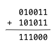
Our result is, . Bits which exist in one element but not the other are combined. Bits that exist in both are canceled out. This is addition in .
We can define a generic addition operation that adds any two numbers of the same type for any field.
gfAdd :: Bits a => a -> a -> a
gfAdd x y =
    x `xor` y
We use the Bits type restriction on the generic type a to ensure that the
xor operation will be defined in the way we expect. Because we have defined
addition in terms of xor, it is relatively easy to prove that subtraction is
the same operation as addition. I leave that as an exercise to the reader. As
a hint, try deriving the additive inverse for any number. Use a truth table.
Polynomial Expansion
Now we can shift our focus to multiplication. Multiplication in a Galois Field
is a little trickier than standard multiplication. We cannot use built-in CPU
operations to help us. A Galois field treats numbers as polynomials. In this
case, the bit position of a number indicates the power. So, for instance, the
number {51} corresponds to 1010001b. This also corresponds to the
polynomial . But, remember that addition in
this field is not the same as addition in
or .
So, the polynomial is really
xor xor . It is this tricky bit that makes the
math we are about to do seem a little different than typical polynomial math.
This also means that we must do multiplication and division the long way. But,
we will optimize things in a bit.
Now that we understand the polynomial representation, we can consider how this
corresponds to the bit pattern of a Word8 or Word32. If each bit represents
a coefficient of the given power of two, then these words make a compact
representation. A Word8 can hold a polynomial of order 8, and a Word32 can
hold a polynomial of order 32. Since we know that xor would cancel out two
terms raised to the same power, a single bit is more than enough storage space
to hold each coefficient, which can be either 1 or 0.
The compact representation cannot be used for any operation other than addition,
because of how binary arithmetic works. Instead, we need to expand this
representation so we can perform multiplications and divisions. This is what
expandPolynomial does.
expandPolynomial :: Word32 -> [Word32]
expandPolynomial x =
        expandPoly 1 x []
    where
        expandPoly 0 _ xs = filter (/=0) xs
        expandPoly y x xs = expandPoly (y `shiftL` 1) x ((y .&. x) : xs)
This function uses the recursive piecewise function expandPoly to build a list
of expanded coefficients. Each of these has exactly one bit set. This is done
by first iterating through all bits in a 32-bit word and performing a bitwise
AND (.&.) using this bit position and the value to be expanded. Each of these
values are pushed onto a list. Finally, when all bits have been iterated, zero
coefficients are removed by using the filter function to retain only non-zero
coefficients from this list.
Polynomial Multiplication
Now we can implement polynomial multiplication. We have a modular step left
before this becomes the multiplication method we will use for this Galois field,
but we will talk about that in a bit. To multiply two values, x and y, we
expand one of the two values and then multiply this expansion by the other
value. This produces a set of intermediate values that must be added
together to get the result. As before, add means xor. To best understand
this operation, think back to how you were taught long-hand multiplication in
grade school. The operation is the same process, more or less.
Consider the following example. We multiply 43 by 19.
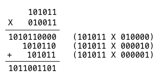
As we can see, the polynomial multiplication of these two numbers is
1011001101b, which corresponds to 717. We multiply the left hand element by a
single bit in the right hand element for each of the bits in the right hand
element. We then add each of these values using xor.
The corresponding function in Haskell is listed here.
polyMult :: Word32 -> Word32 -> Word32
polyMult x y =
    foldl' gfAdd 0 $ map (x*) $ expandPolynomial y
There is a lot going on in this function. First, we use expandPolynomial to
expand y into a list of coefficients. We then use map to multiply x by
each of these coefficients. Finally, we use foldl with gfAdd to collapse
this back into a compact polynomial for this field. The left fold function
repeatedly applies the function in the first argument, gfAdd to each element
in the list, accumulating the result. A more in-depth explanation of foldl is
below in the Low Level Operations section.
Polynomial Multiplication in GF
The polynomial multiplication function as implemented needs some additional work to be closed under multiplication in the field. As we can see with the above example, the value we got from multiplying 43 by 19 is much larger than 255, which is the largest element in our field. Our field is therefore not closed under the multiplication function we have written above. It is possible to use this function with two elements to get an element not in the field. In order to get around this problem, we need to select a prime number that we can use to make this field modular. This means that if we generate an element through multiplication that is not an element in the field, we divide this element by a fixed prime number. The remainder of this division becomes the result of this closed multiplication. We repeat this modulus operation until the remainder is in .
AES uses the prime 283. In hex, this is {11b}. The polynomial form is therefore . This number is an irreducible polynomial, which means that it can only be divided by itself and 1 (also, this is the definition of prime). If we multiply two polynomials modulo this value, then our multiplication is closed under . Because this number is prime, the modular field will contain every element in . The explanation of this fact is rather long-winded, but I highly suggest reading up on field theory to understand why this is true. It is what makes algorithms like AES possible.
Just as we used long form multiplication for polynomials, we use long division for dividing polynomials. To get the modulus form, which is really what we are interested in, we perform the division and only keep the remainder. As with long division, we work from the left to the right of the dividend until the remainder is smaller than the divisor. The values that we multiply the divisor by during each step would, when added together, be the quotient. But, it’s only the remainder we care about.
Getting back to our multiplication example, let’s reduce our result, 717, modulo the prime 283. Here, 283 = 100011011b, and 717 = 1011001101b.
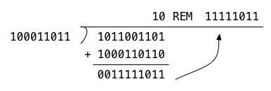
Here, the remainder, which is all we care about for this operation, is
11111011b, or 251. To capture this same operation in Haskell requires some
recursion. We need to find the greatest power of x in the divisor and
dividend, and then find the number we must multiply the divisor by to be less
than or equal to this power. We apply the modulus operation until x is back
in . This could mean applying the operation once
more when x is less than 283 but still greater than 255.
polyRemainder :: Word32 -> Word32 -> Word32
polyRemainder x y =
        if x > 255
            then polyRemainder (gfAdd x factor) y
            else x
    where
        factor = y * (greatestXFactor `div` greatestYFactor)
        greatestXFactor = head $ expandPolynomial x
        greatestYFactor = head $ expandPolynomial y
In this recursive function, we continue execution until x < 256. At this
point, x is the remainder. Through each iteration, we compute the greatest
polynomial factor of both x and y and perform an integer division operation
on these factors. This gives us the factor by which we multiply y to get the
largest multiple of y that we can “subtract” from x for the given coefficient.
The process is very similar to computing a CRC.
Now, we can define gfMult.
gfMult :: Word32 -> Word32 -> Word32
gfMult x y = (flip polyRemainder) 283 $ polyMult x y
In this function, we just take the remainder of the polynomial multiplication of
x and y, which gives us ( x · y ) mod 283.
Multiplicative Inverse
The next thing we are interested in obtaining for the AES algorithm is the multiplicative inverse for any given number in . Now, we could perform an extended Euclidean algorithm to build a function that does this, but there is a much easier way. The functions we have defined so far can be used to build multiplication tables. With some inverted mapping, we can use these tables to derive the multiplicative inverses for any value in the field. Since most AES implementations use table lookups for performing multiplications within the fields, we can kill two birds with one stone. We can build these tables, which can be used for efficient implementations, and we can use these tables to compute the inverse mapping.
First, let’s build a multiplication table. This table is 256 x 256,
and covers multiplying any element by any other element. We use Data.Array
to build a fixed length array of arrays. There are 256 arrays, each of
which contain 256 elements.
multArray :: Array Word8 (Array Word8 Word8)
multArray =
    array (0, 255)
        [(fromIntegral j,
            array (0,255)
                    [(fromIntegral i, fromIntegral $ i `gfMult` j)
                    | i <- [0..255]])
            | j <- [0..255]]
Here, we use list comprehension to define lists of pairs of elements. Each pair
contains the offset in the array to which value (the second argument of the
pair) is stored. The outer list defines offsets for each of the element arrays,
and then defines each element array. The inner list holds the definition of
elements in the element array and their offsets. This is just one giant
multiplication table, like we used to make in grade school. Note the
applications of fromIntegral. The gfMult operation operates on Word32
values. We did this for simplicity, but we actually only care about Word8
values. To help Haskell with some type inference, we use fromIntegral to tell
Haskell where we want Word8 values. This allows Haskell to treat i and j
as Word32 values, which are required for gfMult. Haskell is a strongly
typed language, and will not perform implicit conversions, unlike C, C++, or
Java.
Now, let’s make an optimization. The old way of multiplying in
required using gfMult which had to first do long
multiplication and then long division to perform the modulus operation. This
multiplication table has already performed this work for us. So, we can
optimize this function and call it gfMult'.
gfMult' :: Word8 -> Word8 -> Word8
gfMult' x y = (multArray ! x) ! y
To perform our multiplication, we look up the result in the multiplication
table. The (!) operator is used to select an element at the given offset. We
use the x offset to select the correct element array for multiples of x, and
we use the y offset to select the yth multiple. The advantage of this
multiplication is that it runs in constant time, unlike the original
multiplication operation.
Now, let’s find the multiplicative inverse for each element. First, let’s double-check our definitions. There are two special elements for multiplication. The first element is 0. Anything multiplied by 0 is 0. The second is 1. This element is known as the multiplicative identity. Anything multiplied by 1 is itself. Both of these special elements are immune to this inverse operation. The multiplicative inverse is an element that, when multiplied by the original element, results in the multiplicative identity, the element 1. So, 0 is exempt because it does not have an inverse. There is no number that we can multiply 0 by to get 1. The identity element 1 is exempt because it is its own identity. 1 · 1 = 1.
For simplicity, the first two elements in our inverse list will be 0 and 1. This isn’t exactly accurate, but for our use, it should be fine. Now, for each offset in the multiplication table, we are going to find the offset that holds the element 1. This offset becomes the multiplicative inverse for the given offset.
inverseArray :: Array Word8 Word8
inverseArray =
    array (0, 255)
          ([(0,0), (1,1)]
           ++ [(i,j) | i <- [2..255], j <- [2..255], (gfMult' i j) == 1])
This list is pretty straight-forward. We start with the 0 and 1 elements. As
above, these remain constant. Then, we build a list comprehension in which we
find the value j that, when multiplied by i in
results in
the identity element 1. We know that our multiplication table already contains
all possible elements (otherwise, we’ve introduced a defect), so we simply
iterate through this table to find the correct value.
Now we can build the inverse multiplication table. This is the “division”
table, which allows us to divide the first offset by the second offset. All we
need to do is re-order the multArray using this inverseArray.
divArray :: Array Word8 (Array Word8 Word8)
divArray =
    array (0, 255)
        [(j,
            array (0,255)
                    [(i, j `gfMult'` (inverseArray ! i))
                    | i <- [0..255]])
            | j <- [0..255]]
This divArray allows us to define, for the first time, a complete division
operator for .
gfDiv' :: Word8 -> Word8 -> Word8
gfDiv' x y = (divArray ! x) ! y
As before, this operation runs in constant time. Because of the overhead of
computing inverseArray, the first division will take a long time. Haskell is
a lazy computing language. It does not perform computations until it is forced
to. Subsequent divisions will run in constant time.
For completion sake, we will also define gfAdd' which also operates on 8-bit
words.
gfAdd' :: Word8 -> Word8 -> Word8
gfAdd' x y = x `xor` y
This allows us to operate within using 8-bit words and table based operations. In fact, we can now perform all four operations: addition, subtraction (the same as addition), multiplication, and division. Our Galois field is complete and ready for AES.
Low Level Operations
Before continuing with building up the individual steps in the cipher, we need
to define some low-level conversions. AES is a block cipher. This means that
it operates on a fixed size block of input data at a time. The block size for
AES is 128 bits, which is four 32-bit words or 16 8-bit bytes. We start by
defining an octets function which converts a 32-bit word into 8-bit bytes.
octets :: Word32 -> [Word8]
octets i =
    [ fromIntegral $ i `shiftR` 24
    , fromIntegral $ i `shiftR` 16
    , fromIntegral $ i `shiftR` 8
    , fromIntegral i
    ]
Let’s decompress this function. Based on the signature, we can see that we are
converting a Word32 into a list of Word8 values. The definition of this
function uses repeated fromIntegral calls and shiftR calls to create a list
of Word8 bytes. The shiftR method takes two arguments: an integer to shift,
and the number of positions that it should be bit shifted to the right. The
back ticks around the shiftR function cause it to be treated as an infix
operator (think 1 + 1). The application here of fromIntegral might seem like
a bit of magic. Haskell uses type inference to know that each element of the
list must be of type Word8, while the result type of the shift is a Word32.
Hence, it chooses an application of the generic fromIntegral method that
converts from Word32 to Word8.
To convert to a 32-bit word from a list of octets, we define fromOctets.
Here, we use a left fold to repeatedly shift left and or in the next byte. As
is obvious from both the function above and this function, we are working in
Big Endian mode.
fromOctets :: [Word8] -> Word32
fromOctets = foldl' shiftOp 0
    where shiftOp l b = (l `shiftL` 8) .|. (fromIntegral b)
First, let’s explain foldl. The type signature of foldl is as follows:
foldl :: (a -> b -> a) -> a -> [b] -> aThis function takes three arguments. The first argument is a function that
creates an a result from two arguments, an a and a b. The second argument
is an initial a value. The third argument is a list of b arguments.
foldl produces a result of a that is created by “folding” the list through
repeated applications of the function. The first application takes the a
argument as provided and the first b value from the list. This results in a
new a value, which is used for the next invocation of the function along with
the next b value from the list. Because it takes values from left to right in
the list, it is a left fold. There is also a foldr version that takes values
from right to left.
Getting back to fromOctets, we can see that the function passed to foldl
shifts the current result left by 8 bits and then performs a bitwise-or to fold
in the next byte. Here, fromIntegral converts 8-bit Word8 values to 32-bit
Word32 values. Folding this function effectively undoes what octets does,
as we would expect.
Plaintext and Ciphertext
We define Plaintext and Ciphertext as newtype wrappers around [Word8]
arrays so we can build functions that cleanly operate on either plaintext or
ciphertext data.
newtype Plaintext = Plaintext [Word8]

newtype Ciphertext = Ciphertext [Word8]
This allows us to write function signatures that clearly define what the operations will be doing.
Key
We define a Key type that is used for storing the three distinct key types
supported by AES: 128 bits, 192 bits, and 256 bits. First, we create a RawKey
that is just a thin newtype wrapper around [Word32].
newtype RawKey = RawKey [Word32]Now we can define a Key type which supports one of the three NIST approved key sizes.
data Key = Key128 RawKey | Key192 RawKey | Key256 RawKeyNow in places where we need to treat the key type specially, we can do so by using pattern matching. In places where we just need to get access to the raw key, we provide the following conversion function:
keyToRawKey :: Key -> RawKey
keyToRawKey (Key128 raw) = raw
keyToRawKey (Key192 raw) = raw
keyToRawKey (Key256 raw) = raw
The inverse allows us to map a raw key to the appropriate key type.
rawKeyToKey :: RawKey -> Key
rawKeyToKey raw@(RawKey keyBytes) =
    case length keyBytes of
        4 -> Key128 raw
        6 -> Key192 raw
        8 -> Key256 raw
Here, 4 words correspond to 128 bits, 6 words correspond to 192 bits, and 8 words correspond to 256 bits.
Finally, we will need to consider a KeySchedule as a special type. We create
a newtype wrapper around [Word32] to make our intentions clear when we
manipulate key schedules.
newtype KeySchedule = KeySchedule [Word32]
    deriving (Eq, Show)
We define a default key schedule that does nothing. It is an infinite list of zeros.
defaultKeySchedule :: KeySchedule
defaultKeySchedule = KeySchedule $ repeat 0x00000000
Now we can build functions that make a little more sense from their argument types.
State Array
As per the AES specification, we can now create a state array. This is an array
of four columns representing the current 128-bit state of the cipher. We
express this array as four 32-bit words, named w0, w1, w2, and w3. We
also include a key schedule array, which will be explained later. Here is the
data type.
data State = State {
                w0 :: Word32,
                w1 :: Word32,
                w2 :: Word32,
                w3 :: Word32,
                schedule :: KeySchedule }
    deriving (Eq, Show)
We need a function that loads the state array with input bytes. The
plaintextToState method performs this operation using the low-level routines
provided above.
plaintextToState :: Plaintext -> State
plaintextToState (Plaintext ws) =
        State firstWord secondWord thirdWord fourthWord defaultKeySchedule
    where
        makeWord xs = fromOctets $ take 4 xs
        firstWord  = makeWord ws
        secondWord = makeWord $ drop 4  ws
        thirdWord  = makeWord $ drop 8  ws
        fourthWord = makeWord $ drop 12 ws
take and drop create new lists with the number of taken elements or the
first N elements removed, respectively.
The stateToCiphertext method performs the opposite operation. Here, the ++
operator performs list concatenation. This function is how we get bytes back
out of our State type when we are done with the block cipher.
stateToCiphertext :: State -> Ciphertext
stateToCiphertext (State w0 w1 w2 w3 _) =
        Ciphertext $ (octets w0) ++ (octets w1) ++ (octets w2) ++ (octets w3)
This allows us to focus on writing operations in this cipher as functions
that map values in our State space type onto itself.
AES Operations
There are four operations that we perform during AES rounds. In most of these
rounds, we perform all four of these operations. In the last round, we perform
only three. These operations are SubBytes, ShiftRows, MixColumns, and
AddRoundKey. To build up each of these operations, we will need to build upon
the math and low-level operations we have defined so far to apply these towards
each of these higher level operations.
SubBytes
The SubBytes transformation is a non-linear byte substitution that is
performed on each byte in the State. The byte is substituted with the
multiplicative inverse and then the following affine transformation is applied
to each bit of the byte (from the NIST document):
bi’ = bi + b(i+4) mod 8 + b(i+5) mod 8 + b(i+6) mod 8 + b(i+7) mod 8 + ci
Here, c is the constant {63}. This logic is very easy to implement in code.
We can build up this substitution by mapping the inverseArray with the
transformation as defined in the specification. We create a subBytesArray
that we can use to look up the complete substitution.
subBytesArray :: Array Word8 Word8
subBytesArray =
        array (0, 255) [(i, affineXform $ inverseArray ! i) | i <- [0..255]]
    where
        c = 0x63
        affineXform b =
                    b
            `xor`  (b `rotateR` 4)
            `xor`  (b `rotateR` 5)
            `xor`  (b `rotateR` 6)
            `xor`  (b `rotateR` 7)
            `xor`   c
To simplify things, we create a subByte function which performs the
substitution on a single byte.
subByte :: Word8 -> Word8
subByte x = subBytesArray ! x
With the lookup in the array, this is a constant time operation.
Next, we build a subWord helper function that performs the subByte operation
on each byte in a given Word32.
subWord :: Word32 -> Word32
subWord w32 =
    fromOctets $ map subByte $ octets w32
Here, we split the Word32 value into a list of Word8 octets, map the
subByte operation over this list, and re-combine the resultant map back into a
single Word32 value.
Now, we can build the subBytes routine, which operates in the State space.
subBytes :: State -> State
subBytes st@(State w0 w1 w2 w3 _) =
        st { w0 = (subWord w0),
             w1 = (subWord w1),
             w2 = (subWord w2),
             w3 = (subWord w3) }
This routine builds a new State value in which each word in the state has been
replaced by the subWord of the original word. With that, we have one
operation for each round of AES done.
ShiftRows
In the ShiftRows operation, we shift the rows of the state. Keep in mind that
each word in the state is a column. So, in this operation, we are exchanging
bytes between columns to diffuse data. The first row is left unchanged. The
second row is rotated to the left by 1. The third is rotated to the left by 2.
The fourth is rotated to the left by 3.
shiftRows :: State -> State
shiftRows st@(State w0 w1 w2 w3 _) =
        shift (octets w0) (octets w1) (octets w2) (octets w3)
    where
        shift ([w00,w01,w02,w03]) ([w10,w11,w12,w13])
              ([w20,w21,w22,w23]) ([w30,w31,w32,w33]) =
                    st { w0 = (fromOctets [w00,w11,w22,w33]),
                         w1 = (fromOctets [w10,w21,w32,w03]),
                         w2 = (fromOctets [w20,w31,w02,w13]),
                         w3 = (fromOctets [w30,w01,w12,w23]) }
Here, we use octets to expand each column, and then use pattern matching in
the shift helper function to grab each byte. From there, we can perform the
row level shifting for each column, and then recombine these into Word32
values using fromOctets. Compared to SubBytes, ShiftRows is relatively
easy. In fact, it’s the simplest of the four steps.
MixColumns
The MixColumns operation is where things get interesting. This is the core
diffusion operation in AES. The code itself is simple, but understanding what
the code is doing requires some explanation. The ShiftRows operation shifted
bytes between columns to diffuse data within the block. The MixColumns
operation will perform some multiplications of bytes within each column over
multiplying them with a special polynomial , modulo the polynomial . I will explain
why this polynomial is special in a bit. If we treat each byte in a column,
say, s0, s1, s2, and s3 as a polynomial as well, then we get . Now we can derive the math necessary to build the
MixColumns algorithm. This will be the second longest derivation in the
article, so bear with me. The math is actually quite beautiful, which is why
I’m showing it.
Let’s expand this operation by multiplying through:
At this point, we have a sixth order polynomial, which is three orders too large. To resolve this, we take the remainder of division by . On each line, we will “subtract” a multiple of this reducing polynomial and simplify the result on the next line. Keep in mind that addition and subtraction are the same thing. We use the minus signs just to show the multiple during each step of our modulo reduction.
This gives us our final polynomial. As the reduction modulo occurs,
note that terms missing for each factor are added back in. This is a beautiful
application of a reducing polynomial. Based on this math, we know exactly which
values should be xored into each byte for the MixColumns operation.
As per the reduction above, we will perform the following operations on each byte in the column. I have re-arranged the order of the bytes to match what is found in the NIST documentation. We can see that our derivation matches the implementation documentation exactly. If you read the above equation from bottom up, right to left, and these sets of equations from top down, left to right, the coefficients are the same.
We shall begin by building four simple Haskell functions that reproduce the
result for each byte in MixColumns.
mixCol0 :: Word8 -> Word8 -> Word8 -> Word8 -> Word8
mixCol0 s0 s1 s2 s3 =
                 (0x02 `gfMult'` s0)
        `gfAdd'` (0x03 `gfMult'` s1)
        `gfAdd'` (0x01 `gfMult'` s2)
        `gfAdd'` (0x01 `gfMult'` s3)

mixCol1 :: Word8 -> Word8 -> Word8 -> Word8 -> Word8
mixCol1 s0 s1 s2 s3 =
                 (0x01 `gfMult'` s0)
        `gfAdd'` (0x02 `gfMult'` s1)
        `gfAdd'` (0x03 `gfMult'` s2)
        `gfAdd'` (0x01 `gfMult'` s3)

mixCol2 :: Word8 -> Word8 -> Word8 -> Word8 -> Word8
mixCol2 s0 s1 s2 s3 =
                 (0x01 `gfMult'` s0)
        `gfAdd'` (0x01 `gfMult'` s1)
        `gfAdd'` (0x02 `gfMult'` s2)
        `gfAdd'` (0x03 `gfMult'` s3)

mixCol3 :: Word8 -> Word8 -> Word8 -> Word8 -> Word8
mixCol3 s0 s1 s2 s3 =
                 (0x03 `gfMult'` s0)
        `gfAdd'` (0x01 `gfMult'` s1)
        `gfAdd'` (0x01 `gfMult'` s2)
        `gfAdd'` (0x02 `gfMult'` s3)
Now, we can put all of this together into a mixColumns function.
mixColumns :: State -> State
mixColumns st@(State w0 w1 w2 w3 _) =
        st { w0 = (mixOctets w0),
             w1 = (mixOctets w1),
             w2 = (mixOctets w2),
             w3 = (mixOctets w3) }
    where
        mixOctets w32 = mix $ octets w32
        mix ([s0,s1,s2,s3]) =
            fromOctets
                    [ mixCol0 s0 s1 s2 s3
                    , mixCol1 s0 s1 s2 s3
                    , mixCol2 s0 s1 s2 s3
                    , mixCol3 s0 s1 s2 s3]
At this point, we can perform three of the four steps in an AES round. We’ve
almost derived everything we need to understand how MixColumns
works. But, there is still something we haven’t delved into. What was that
polynomial,
about?
In order to diffuse data between columns, a linear operation was required in AES. The operation needs to “mix” things up, but it needs to do so in a way that can be reversed during decryption. The polynomial used for the mix operation is a different representation of an invertible matrix in . The operation on the bytes in the column can also be represented by a square matrix. We can form a circulant matrix from this polynomial. The circulant matrix is as follows:
Square matrices are either singular or invertible. The way to tell the
difference is to take the determinant of the matrix. If a square matrix has a
non-zero determinant, then it also has an inverse. We can use that inverse to
derive the polynomial which undoes the MixColumns operation. Let’s take the
determinant of this matrix. Again, addition and subtraction are just customary
for this operation, representing the parity of cofactors. They still mean the
same thing in this field, and will be applied as xors.
Therefore, this matrix is invertible. We can find the inverse through Gauss-Jordan elimination. We’ll start by creating an augmented matrix, which will allow us to keep track of all of the operations necessary to invert our circulant matrix. When we are done, we will have the identity matrix augmented with the inverse of our matrix.
First, we multiply each row by the inverse necessary to turn its pivot column
into a unit value. This inverse is computed in
using the
inverseArray we created earlier. Inverting these pivot columns ahead of time
greatly simplifies the elimination computations below.
Next, we subtract from and , and from . goes along for the ride.
Now we normalize the pivot for . All other rows go along for the ride.
Next, we cancel out in each of the other three rows.
Next, we cancel out in each of the other three rows.
Then, we normalize . If everything goes right, we should see the coefficients of our new polynomial appear in ’s augmented row.
Now, we just propagate this change through the rest of the matrix to get our inverse matrix.
This is the matrix that undoes MixColumns when we decrypt:
The designers of AES were careful to select a square matrix that was invertible
over this field. Repeating this inversion operation may have seemed tedious,
but I wanted to demonstrate the math behind the construction of this step.
It is a very interesting application of matrix math, and it shows how we can
build upon known algebraic techniques in more exotic fields.
As a side-note, there are
other possible polynomials that could be used for mixing columns. These
polynomials would be incompatible with AES, but as long as one selects an
invertible polynomial and derives the inverse, one could perform this
substitution. It’s difficult to predict the effects that such a change would
have on the security of the cipher, but it’s a possible avenue of exploration
for the adventurous. The math that I have demonstrated here could be used to
derive a different set of polynomials for the MixColumns step.
Simple pattern matching between the two matrices will make the inverse
MixColumns polynomial for AES obvious.
It’s
.
I will leave the derivation
of the inverse MixColumns operation as an exercise for the reader. It should
be a simple application of the steps that I went over from the start of this
section until the last Haskell function derived above. Now, let’s get back to
encryption.
Key Expansion
Before we can delve into AddRoundKey, we will need to build up some code that
can perform AES key expansion. During each AddRoundKey call, the current key
schedule for a given round is added into the current AES state. Without the
key, AES is simply a poor hash algorithm. It is the key which adds “confusion”
to the “diffusion”.
We can think of the key schedule as an infinite list that starts with the raw bytes of the key, and continues with values that have been expanded through an algorithm meant to mix these bits for additional rounds of the AES cipher. We will build this function from the ground up by building components necessary for the key expansion process. We can then easily compose the full key expansion function.
We re-use the subWord function that we created in the SubBytes step. We
also create a rotWord function that rotates all of the bytes in a given word
once to the left.
rotWord :: Word32 -> Word32
rotWord w =
        rotate $ octets w
    where
        rotate [w0, w1, w2, w3] = fromOctets [w1, w2, w3, w0]
Next, we need to define the Rcon list. This is a list of words from 1 to N
where each word is made up of the following octets:
. Here, is defined as
. The following Haskell function captures this list.
rcon :: [Word32]
rcon =
    map toWord32 $ iterate (0x02 `gfMult'`) 0x01
  where
    toWord32 w8 = fromOctets [w8, 0, 0, 0]
Haskell already has a high-level function, called iterate, which we can use to
generate the Rcon list. The first argument to this function is a function
that should be applied during each iteration. The second argument is the value
to use for the first iteration. iterate performs the following piece-wise
function:
Here, a0 refers to the second argument of iterate. Based on our
use, this means that Rcon will iterate through the powers of over
.
This is defined as an infinite list, but we know by the
properties of
that the sequence will repeat every 256 entries.
Before we build the key expansion operation, we need some helper types that will
help to keep our intentions clear as we define various functions. We need
KeyLength, Index, and KeyWord, which correspond to the length
of our key in words, the index into the key schedule, and a word in this key
schedule, respectively.
newtype KeyLength = KeyLength Int
    deriving (Eq, Show)
newtype Index = Index Int
    deriving (Eq, Show)
newtype KeyWord = KeyWord Word32
    deriving (Eq, Show)
The key expansion operation is similar for 128, 192, and 256 bit keys. The
first N words is the key itself. Afterward, a sequence of N words is generated
from these words by xoring a previous word in the sequence with the previous
value. Every N words, this temporary value is rotated and inverted. In the
case of a 256-bit key, every N/2 words, the temp value is inverted. Now we can
define the key expansion list. The following function performs expansion of a
key defined as a list of Word32 values. We will create a generic
parameterized function which expands the key based on parameters we provide, and
then we will define a concrete key expansion function for each of the 3
NIST-approved key lengths.
keyExpand :: RawKey -> (KeyLength -> Index -> KeyWord -> Word32 -> Word32)
              -> KeySchedule
keyExpand raw@(RawKey key) subFunc =
        KeySchedule $
            key ++ (expandedKey keyLength (last key) $ keyExpand raw subFunc)
    where
        keyLength = length key
        expandedKey i temp (KeySchedule (k:ks)) =
            let newTemp =
                    (subFunc (KeyLength keyLength) (Index i) (KeyWord k) temp)
            in newTemp : expandedKey (i + 1) newTemp (KeySchedule ks)
We can compose the expansion substitution function from some small building
blocks. First, we have the basic xor with the previous value step that
happens during the non-special steps. Here, we just re-use the generic gfAdd
function.
xorWords :: Word32 -> Word32 -> Word32
xorWords = gfAdd
The second building block is the major rotation / substitution operation that happens every N words.
rotateSubWord :: KeyLength -> Index -> KeyWord -> Word32 -> Word32
rotateSubWord (KeyLength keyLength) (Index i) (KeyWord w) temp =
    flip xorWords w $
        xorWords
            (subWord (rotWord temp))
            (rcon !! ((i `div` keyLength) - 1))
Finally, for 256-bit keys, we provide subTemp which performs a subWord on
temp prior to the xorWords operation.
subTemp :: Word32 -> Word32 -> Word32
subTemp temp w =
    xorWords (subWord temp) w
Now, we can put this all together into a key expansion operation for AES-128.
subFuncAes128 :: KeyLength -> Index -> KeyWord -> Word32 -> Word32
subFuncAes128 kl@(KeyLength keyLength) ind@(Index i) kw@(KeyWord k) temp =
    if (i `mod` keyLength) == 0
        then rotateSubWord kl ind kw temp
        else xorWords temp k
The key expansion operation for AES-192 is exactly the same operation.
subFuncAes192 :: KeyLength -> Index -> KeyWord -> Word32 -> Word32
subFuncAes192 = subFuncAes128
Finally, we can compose the AES-128 key expansion operation plus an additional
if/then/else block to build the AES-256 substitution operation.
subFuncAes256 :: KeyLength -> Index -> KeyWord -> Word32 -> Word32
subFuncAes256 kl@(KeyLength keyLength) ind@(Index i) kw@(KeyWord k) temp =
    if ((0 == i `mod` (keyLength `div` 2)) && (0 /= i `mod` keyLength))
        then xorWords (subWord temp) k
        else subFuncAes128 kl ind kw temp
Now, we have substitution functions for each of the key lengths. Let’s define the key expansion operations for each cipher.
nistKeyExpand :: Key -> KeySchedule
nistKeyExpand (Key128 raw) = keyExpand raw subFuncAes128
nistKeyExpand (Key192 raw) = keyExpand raw subFuncAes192
nistKeyExpand (Key256 raw) = keyExpand raw subFuncAes256
This function selects the correct key expansion operation based on the length of
the key. Note that we did not define a general case nistKeyExpand function.
A runtime error will occur if we attempt to use a key size that has not been
defined by NIST.
AddRoundKey
The last step that we have to define is the AddRoundKey step. This uses the
key schedule that we developed in the last section. We need to first create a
function that adds a given key schedule to the AES state.
setKey :: Key -> State -> State
setKey key st =
    st { schedule = nistKeyExpand key }
This function takes an AES key and a State as input, and returns a new State
with that AES key set. We will assume that this step has been done at the
point of performing the AddRoundKey step.
Now, the addRoundKey function is easy to define.
addRoundKey :: State -> State
addRoundKey st@(State w0 w1 w2 w3 (KeySchedule schedule)) =
    st { w0 = w0 `xor` (schedule !! 0),
         w1 = w1 `xor` (schedule !! 1),
         w2 = w2 `xor` (schedule !! 2),
         w3 = w3 `xor` (schedule !! 3),
         schedule = KeySchedule $ drop 4 schedule }
Each time addRoundKey is called, it adds in four words from the key schedule,
and adjusts the key schedule for the next round. This is returned as a State.
AES Encryption
Before we can write the AES encryption function, we need a function that returns the number of rounds required for a given key. We define it here.
roundsForKey :: Key -> Int
roundsForKey (Key128 _) = 10
roundsForKey (Key192 _) = 12
roundsForKey (Key256 _) = 14
At this point, we have all of the primitive operations and steps defined to perform AES block encryption. The complete operation can be constructed by composing these steps into a recursive function. This set of steps mirrors the pseudocode provided in the NIST documentation, but is written in a functional way. This has the advantage of making it very easy for us to unroll our implementation step-by-step for testing purposes. Also, because we avoid side-effects, we significantly lower the amount of possible defects that are in this implementation as compared to building an equivalent implementation based on the NIST pseudocode.
aesBlockEncrypt :: Plaintext -> Key -> Ciphertext
aesBlockEncrypt input key =
        stateToCiphertext $
            blockCipher (roundsForKey key) $
                        addRoundKey $ setKey key $ plaintextToState input
    where
        blockCipher rounds st =
            if rounds == 1
                then
                    addRoundKey $ shiftRows $ subBytes st
                else
                    blockCipher (rounds - 1) $
                        addRoundKey $ mixColumns $ shiftRows $ subBytes st
There you have it. This function will perform AES encryption, and will successfully pass the test vectors defined in the NIST document. I will expand upon this basic function in my next article, where I will use it to build a parametric pseudo-random number generator.